---
jupytext:
text_representation:
extension: .md
format_name: myst
kernelspec:
display_name: Python 3
language: python
name: python3
---
```{code-cell}
:tags: [remove-input]
import random
random.seed(1028)
import sys
import os
sys.path.append(os.path.abspath(os.path.join(os.getcwd(), '..')))
```
(sec:policy-based:policy-gradients)=
# Policy gradients
````{margin}
```{admonition} Video byte: Introduction to policy gradient methods
```
````
```{admonition} Learning outcomes
The learning outcomes of this chapter are:
1. Apply policy gradients and actor critic methods to solve small-scale MDP problems manually and program policy gradients and actor critic algorithms to solve medium-scale MDP problems automatically.
2. Compare and contrast policy-based reinforcement learning with value-based reinforcement learning.
```
## Overview
````{margin}
```{admonition} Video byte: Intuition of policy gradient methods
```
````
As noted earlier, policy-based methods search for a policy directly, rather than searching for a value function and extracting a policy. In this section, we look at a model-free method that optimises a policy directly. It is similar to Q-learning and SARSA, but instead of updating a Q-function, it updates the parameters $\theta$ of a policy directly using gradient ascent.
In policy gradient methods, we approximate the policy from the rewards and actions received in our episodes, similar to the way we do it with Q-learning. We can do this provided that the policy has two properties:
````{margin}
```{admonition} Video byte: Policy gradients
```
````
1. The policy is represented using some function that is **differentiable** with respect to its parameters. For a non-differentiable policy, we cannot calculate the gradient.
2. Typically, we want the policy to be **stochastic**. Recall from the section on [policies](sec:mdps:policies) that a stochastic policy specifies a **probability distribution** over actions, defining the probability with which each action should be chosen.
The goal of a policy gradient is to approximate the optimal policy $\pi_{\theta}(s, a)$ via gradient ascent on the expected return. Gradient ascent will find the best parameters $\theta$ for the particular MDP.
## Policy improvement using gradient ascent
````{margin}
```{admonition} Video byte: Intuition of policy gradients
```
````
The goal of gradient ascent is to find weights of a policy function that maximises the expected return. This is done iteratively by calculating the gradient from some data and updating the weights of the policy.
The [expected value](defn:expected-discounted-reward) of a policy $\pi_{\theta}$ with parameters $\theta$ is defined as:
$$J(\theta) = V^{\pi_{\theta}}(s_0)$$
where $V^{\pi_{\theta}}$ is the policy evaluation using the policy $\pi_{\theta}$ and $s_0$ is the initial state. This expression is computationally expensive to calculate, because we need to execute every possible episode from $s_0$ to every terminal state, which may be an infinite number of episodes. So, we use policy gradient algorithms to approximate this instead. These search for a local maximum in $J(\theta)$ by **ascending the gradient** of the policy with respect to the parameters $\theta$, using episodic samples.
:::{admonition} Definition -- Policy gradient
Given a policy objective $J(\theta)$, the **policy gradient** of $J$ with respect to $\theta$, written $\nabla_{\theta}J(\theta)$ is defined as:
$$
\nabla_{\theta}J(\theta) = \begin{pmatrix} \frac{\partial J(\theta)}{\partial \theta_1} \\ \vdots \\ \frac{\partial J(\theta)}{\partial \theta_n} \end{pmatrix}
$$
where $\frac{\partial J(\theta)}{\partial \theta_i}$ is the partial derivative of $J$ with respective to $\theta_i$.
:::
If we want to follow the gradient towards the optimal $J(\theta)$ for our problem, we use the gradient and update the weights:
$$\theta \leftarrow \theta + \alpha \nabla J(\theta)$$
where $\alpha$ is a learning rate parameter that dictates how big the step in the direction of the gradient should be.
The question is: what is $\nabla J(\theta)$? The **policy gradient theorem** (see Sutton and Barto, Section 13.2) says that for any differentiable policy $\pi_{\theta}$, state $s$, and action $a$, that $\nabla J(\theta)$ is:
$$\nabla J(\theta) = \mathbb{E}[\nabla\ \textrm{ln} \pi_{\theta}(s, a) Q(s,a)]$$
The expression $\textrm{ln} \pi_{\theta}(s, a)$ tells us how to change the weights $\theta$: increase the log probability of selecting action $a$ in state $s$. If the quality of selecting action $a$ in $s$ is positive, we would increase that probability; otherwise we decrease the probability.
So, this is the expected return of taking action $\pi_{\theta}(s,a)$ multiplied by the gradient.
In these notes, we will not go into details about gradients or algorithms for solving them -- this is itself a large topic that is relevant outside of reinforcement learning. Instead, we will just give the intuition and how to use this for model-free reinforcement learning.
## REINFORCE
````{margin}
```{admonition} Video byte: REINFORCE
```
````
The REINFORCE algorithm is one algorithm for policy gradients. We cannot calculate the gradient optimally because this is too computationally expensive -- we would need to solve for all possible trajectories in our model. In REINFORCE, we sample trajectories, similar to the sampling process in [Monte-Carlo reinforcement learning](sec:model-free:monte-carlo-learning).
```{figure} ./figs/policy_gradient_loop.png
---
name: fig:policy_gradient_loop
alt: "An abstract illustration of the policy gradient algorithm REINFORCE. There are three boxes: environment, update policy, and sample action. From sample action to environment is an arrow labelled with the letter a, representing the action being executed by the agent in the environment. From the environment back to select action is an arrow labelled s-prime. This indicates the REINFORCE iteratively selects and executes actions. From environment, there are two arrows labelled r and s, each with short arrows above them illustrating that these are lists or vectors of rewards and states. The arrow is also labelled terminated episode, indicating that when an episode terminates, the list of rewards and states are given to the agent, which uses them to update the policy."
---
An abstraction illustration of the policy gradient algorithm REINFORCE.
```
{numref}`fig:policy_gradient_loop` gives an abstract overview of REINFORCE. The algorithm iteratively generates new actions by sampling from its policy and executes these. Once an episode terminates, a list of the states, actions, and rewards is used to update the policy, showing that the policy is only updated at the end of each episode.
```{prf:algorithm} REINFORCE
:label: algorithm:reinforce
$
\begin{array}{l}
\alginput:\ \text{A differentiable policy}\ \pi_{\theta}(s,a),\ \text{an MDP}\ M = \langle S, s_0, A, P_a(s' \mid s), r(s,a,s')\rangle\\
\algoutput:\ \text{Policy}\ \pi_{\theta}(s,a)\\[2mm]
\text{Initialise parameters}\ \theta\ \text{arbitrarily}\\[2mm]
\algrepeat\ \text{(for each episode}\ e \text{)}\\
\quad\quad \text{Generate episode}\ (s_0, a_0, r_1, \ldots s_{T-1}, a_{T-1}, r_{T})\ \text{by following}\ \pi_{\theta}\\
\quad\quad \algforeach\ (s_t, a_t)\ \text{in the episode}\\
\quad\quad\quad\quad G \leftarrow \sum_{k=t+1}^{T} \gamma^{k-t-1} r_k\\
\quad\quad\quad\quad \theta \leftarrow \theta + \alpha \gamma^{t} G\ \nabla\ \textrm{ln}\ \pi_{\theta}(s_t,a_t)\\
\alguntil\ \pi_{\theta}\ \text{converges}
\end{array}
$
```
REINFORCE generates an entire episode using Monte-Carlo simulation by following the policy so far by sampling actions using the stochastic policy $\pi_{\theta}$. It samples actions based on their probabilities; that is, $a \sim \pi_{\theta}(s,a)$.
It then steps through each action in the episode, and calculates $G$, the total future discounted reward of the trajectory. Using this reward, it calculates the gradient $\pi$ and multiples this in the direction of $G$. Therefore, it generates better and better policies as $\pi$ is improved.
````{margin}
```{admonition} Video byte: Convergence
```
````
Comparing to value-based techniques, we can see that REINFORCE (and other policy-gradient approaches) do not evaluate each action in the policy improvement process. In policy iteration, we update the policy $\pi(s) \leftarrow \textrm{argmax}_{a \in A(s)} Q^\pi(s,a)$. In REINFORCE, the most recently sampled action and its reward are used to calculate the gradient and update.
This has the advantage that policy-gradient approaches can be applied when the action space or state space are continuous; e.g. there are one or more actions with a parameter that takes a continuous value. This is because it uses the gradient instead of doing the policy improvement explicitly. For the same reason, policy-gradient approaches are often more efficient than value-based approaches when there are a large number of actions.
:::{note}
From the algorithm above, we can see that REINFORCE is an [on policy](sec:model-free:on-policy-vs-off-policy) approach. The sample trajectories are drawn directly from $\pi_{\theta}$ and the policy is updated at the end of the episode.
:::
(sec:policy-gradients:logistic-regression)=
## Implementation: Logistic regression-based REINFORCE
The implementation of REINFORCE takes a policy, but this policy must be differentiable. As such, we cannot use the tabular policy used in policy iteration. As we can see, unlike Q-learning and SARSA, the update happens only at the end of each episode.
```{code-cell} ipython3
:load: "../mastering_rl/learners/reinforce.py"
```
We need a differentiable policy so that we can calculate the gradient and update. To illustrate this from first principles, let's look at an implementation of a policy that uses logistic regression. This basic implementation supports environments with only two actions, but it is sufficient to illustrate the basics of policy gradient methods from first principles.
Because we use logistic regression to represent the policy in this simplified implementation that allows only two actions, the probability for each action (and therefore the policy) can be calculated as follows:
$$
\begin{aligned}
\pi_{\theta}(s, a_0) &= \frac{1}{1 + e^{-\theta \cdot s}}\\[1mm]
\pi_{\theta}(s, a_1) &= 1 - \pi_{\theta}(s, a_0)
\end{aligned}
$$
This gives us the probability of choosing actions $a_0$ and $a_1$ in state $s$, which approximates the expression $\pi_{\theta}(s, a) Q(s,a)$ in the policy gradient theorem.
Since the policy follows a sigmoid function, we can use the following result from calculus to find the derivative. If $\sigma(x)$ is a sigmoid, then the derivative of $\sigma(x)$ with respect to $x$ conforms to the following pattern:
$$
\begin{aligned}
\sigma(x) &= \frac{1}{1 + e^{-\theta \cdot x}}\\[1mm]
\frac{\partial \sigma(x)}{\partial x} &= \theta \sigma(x)(1 - \sigma(x))
\end{aligned}
$$
Using this result, we can then find $\nabla \textrm{ln} \pi(s, a)$:
$$
\begin{aligned}
\nabla \textrm{ln} \pi_{\theta}(s, a_0) &= s - s\cdot \pi_{\theta}(s, a_0)\\[1mm]
\nabla \textrm{ln} \pi_{\theta}(s, a_1) &= -s \cdot \pi_{\theta}(s, a_0)
\end{aligned}
$$
This gives us a vector of the partial derivatives, which the `update` method then uses to update the corresponding $\theta_i$ value.
Let's implement this.
The policy inherits from `StochasticPolicy`, which means that the policy is a [stochastic policy](sec:mdp:deterministic-vs-stochastic-policies) $\pi_{\theta}(s,a)$ that returns the probability of action $a$ being executed in state $s$. The `select_action` is stochastic, as can be seen below -- it selects between the two actions using the policies probability distribution.
```{code-cell} ipython3
:load: "../mastering_rl/policies/logistic_regression_policy.py"
```
The `update` method, as well as the `gradient_log_pi` method that it calls, are where the policy gradient theorem is applied. In `update`, for every state-action transition in the trajectory, we calculate the gradient and then update the parameters $\theta$ using the corresponding partial derivative.
Let's try this implementation on an example using the REINFORCE algorithm and our logistic regression policy. Because our logistic regression policy supports only two actions, we cannot use the 4x3 GridWorld example, so we instead use an even simpler example (who thought that would be possible!) of a GridWorld that is 11x1 and has a -1 reward at one end and a +1 reward at the other:
```{code-cell} ipython3
from mastering_rl.learners.reinforce import REINFORCE
from mastering_rl.markov_decision_processes.gridworld import GridWorld
from mastering_rl.policies.logistic_regression_policy import LogisticRegressionPolicy
gridworld = GridWorld(
height=1, width=11, initial_state=(5, 0), goals=[((0, 0), -1), ((10, 0), 1)]
)
gridworld_image = gridworld.visualise()
```
Next, we create a `LogisticRegressionPolicy` with just two actions, `left` and `right`, and with two parameters corresponding to the $x$ and $y$ coordinates. This is used in a `REINFORCE` instance to produce the following policy:
```{code-cell} ipython3
policy = LogisticRegressionPolicy(
actions=[GridWorld.LEFT, GridWorld.RIGHT],
num_params=len(gridworld.get_initial_state()),
)
policy_gradient = REINFORCE(gridworld, policy)
policy_gradient.execute(episodes=100)
policy_image = gridworld.visualise_stochastic_policy(policy)
```
We can see here that this is a stochastic policy --- instead of giving us an action (left or right) in each cell, we get the probability that the policy will select each of these actions. The policy learns to select right with a much higher probability because the positive reward is to the right.
To follow the policy, we can use this deterministically by simply selecting the action with the highest probability, but in some applications, the optimal behaviour is to select an action by sampling from the probability distribution.
The difference between value-based methods such as Q-learning and SARSA is demonstrated by the output: there is just a policy and no value function or Q-function because the policy is learnt directly.
If we step through the policy during training, we can see the gradient updates performing their role in policy improvement:
```{only} html
```
This policy only considers two actions, but it can be easily extended to support multiple actions using standard machine learning techniques like one-vs-rest classification.
(sec:policy-gradient:deep-policy-gradients)=
## Implementation: Deep REINFORCE
Just like we can use deep neural networks to approximate Q-functions in [deep Q learning](sec:function-approximation:deep-Q-learning), we can use deep neural networks to approximate policies. Neural networks are differentiable, so these can be used in policy gradient algorithms such as REINFORCE --- the policy parameters $\theta$ are the parameters to the neural network.
As with deep Q learning, this has the advantage that features of the problem are learnt, features do not have to be independent, therefore supporting a larger set of problems compared to a logistic regression approach, and we can use unstructured data as input, such as images and videos.
To implement a deep policy gradient approach in REINFORCE, we just have to implement a new policy that uses a deep neural network.
In our implementation, we again use the PyTorch deep learning framework (https://pytorch.org/).
The policy uses a three layer network with the following:
1. The first layer takes the state vector, so the input features are the features of the state. In the case of the GridWorld example, this would be just the x- and y-coordinates of the agent.
2. We have a hidden layer, with a default number of 64 hidden dimensions, but this is parameterised by the variable `hidden_dim` in the `__init__` constructor.
3. The third and final layer is the output layer, which returns a categorical distribution with a dimensionality the same size as the action space, so that each action is associated with a probability of being selected.
4. We use a non-linear ReLU (rectified linear unit) between layers.
Recall from the section on [deep Q learning](sec:function-approximation:deep-Q-learning) that the `Linear` layers are dense layers in PyTorch.
It inherits from the `StochasticPolicy` and then implement the `update`, `select_action`, and `get_probability` methods. These take advantage of optimisations with the PyTorch framework, so the calculation of the gradient is 'hidden' by the PyTorch library. The line `self.optimiser.zero_grad()` then 'zeros' out the existing gradient so that the new gradient can be calculated. The gradient is calculated using `loss.backwards()`. Then `self.optimiser.step()` adjusts the parameters $\theta$ in the direction of the gradient:
```{code-cell} ipython3
:load: "../mastering_rl/policies/deep_nn_policy.py"
```
As with the [deep Q learning](sec:function-approximation:deep-Q-learning) implementation, PyTorch does not support strings as values, so we need to encode action names and states as integers.
We can now use this implementation by creating a REINFORCE agent with a `DeepNeuralNetworkPolicy` instance as the policy, and use it to learn a policy for the GridWorld example:
```{code-cell} ipython3
:load: "../mastering_rl/tests/_09_policy_gradients/deep_reinforce_run.py"
```
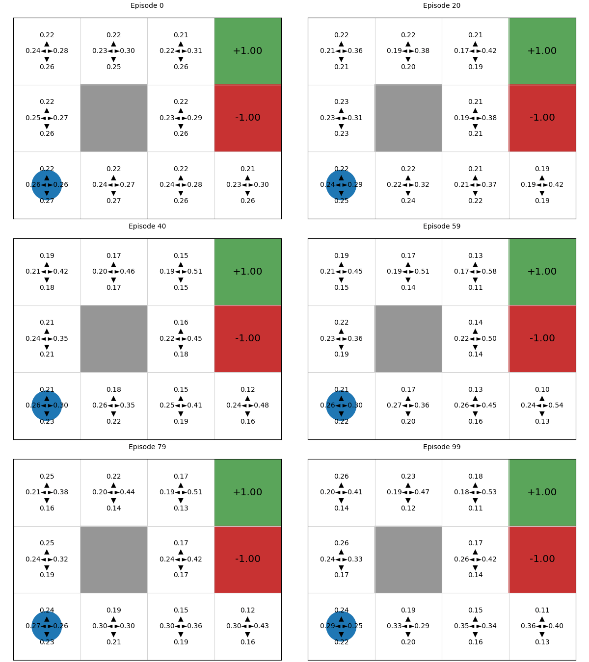
Again, we can see that this policy is stochastic: each action has a probability of being executed in a state.
Simulating the process of training the policy, we can see that initially, all four actions have (approximately) the same probability of being executed, but deep REINFORCE learns a good Q-function and therefore policy:
```{only} html
```
## Advantages and disadvantages of policy gradients (compared to value-based techniques)
### Advantages
- **High-dimensional problems**: The major advantage of policy-gradient approaches compared to value-based techniques like Q-learning and SARSA is that they can handle high-dimensional action and state spaces, including actions and states that are continuous. This is because we do not have to iterate over all actions using $\textrm{argmax}_{a \in A(s)}$ as we do in value-based approaches. For continuous problems, $\textrm{argmax}_{a \in A(s)}$ is not possible to calculate, while for a high number of actions, the computational complexity is dependent on the number of actions.
### Disadvantages
- **Sample inefficiency**: Since the policy gradients algorithm takes an entire episode to do the update, it is difficult to determine which of the state-action pairs are those that effect the value $G$ (the episode reward), and therefore which to sample.
- **Loss of explainability**: Model-free reinforcement learning is a particularly challenging case to understand and explain why a policy is making a decision. This is largely due to the model-free property: there are no action definitions that can used as these are unknown. However, policy gradients are particularly difficult because the values of states are unknown: we just have a resulting policy. With value-based approaches, knowing $V$ or $Q$ provides some insight into why actions are chosen by a policy; although explainability problems still remain.
## Takeaways
```{admonition} Takeaways
- **Policy gradient methods** such as REINFORCE directly learn a policy instead of first learning a value function or Q-function.
- Using trajectories, the parameters for a policy are updated by **following the gradient upwards** -- the same as gradient descent but in the opposite direction.
- Unlike policy iteration, policy gradient approaches are **model free**.
```